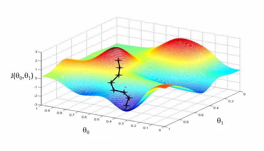
Gradient descent is an optimization algorithm for finding the minimum of a function. It takes steps proportional to the negative of the gradient to find the local minimum of a function. The following 3D figure shows an example of gradient descent. theta1 and theta0 are the two paramters. Gradient descent tries to find one of the local minima.
Gradients really become meaningful in multivarible functions, where the gradient is a vector of partial derivatives. With single variable functions, the gradient is a one dimensional vector with the slope as its single coordinate (so, not very different to the slope at all).
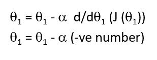
The algorithm for gradient descent is shown as follows. The parameters are simultaneously updated.
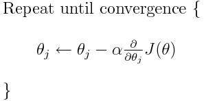
The hyperparamter alpha is called learning rate. It is length of the step taken from every point to reach the local minima.
The first order derivative of a function gives the slope at that particular point.
Algorithm Explained
Let's look at an example and understand the gradient descent algorithm. Consider a linear equation as shown below. theta1 and theta0 are the two paramters. I will use theta wording instead of symbol.
There are many cost functions. In our case of linear equation, our purpose is to reduce the mean squared error between the hypothesis (h(x)) value and actual value.The cost function is shown as follows
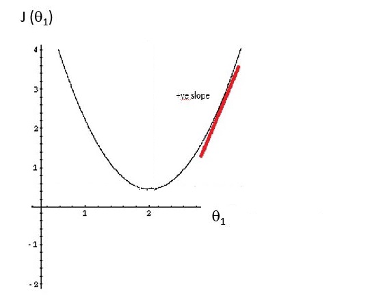
The following figure shows plot between J(theta1), theta1 and a tangent line (shown in red) that has a positive slope, and therefore has a positive derivative.
In gradient descent the theta1 is updated as theta1, minus alpha times some positive number.The Alpha i.e the learning parameter, is always a positive number.So,the theta1 is updated as theta 1 minus something and therefore end up moving theta one to the left. This decreases theta one, and helps in moving towards the direction of the minimum.
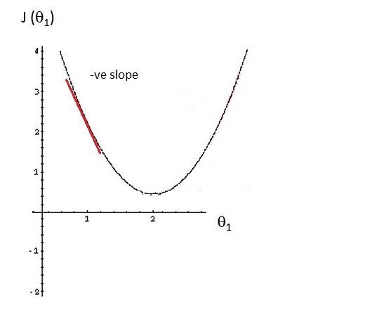
Let's look at the negative slope tangent line. The following figure shows a tangent line (shown in red) that has a negative slope, and therefore has a negative derivative.
The theta 1 is updated as theta 1, minus alpha times some negative number. The Alpha i.e the learning parameter is always a positive number. So, the theta 1 is updated as theta 1 plus something and therefore end up moving theta one to the right. This increases theta one and helps in moving towards the direction of the minimum.
The learning parameter (alpha) value determines how fast or slow the gradient descent will be. If it is too small gradient descent will be slow. If it is too large then gradient descent will overshoot and may fail to converge.
What if theta 1 is already at local minima?
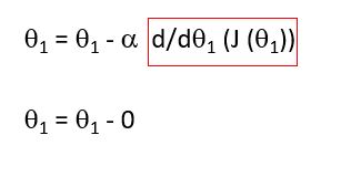
At the local optimum,the derivative will be equal to zero. So, the slope of this line will be equal to zero and thus this derivative term is equal to zero. If we are already at the local optimum it leaves theta 1 unchanged cause its updates as theta 1 equals theta 1. Therefore the solution remains at the local optimum.
How gradient descent finds local optima when there are many local optima?
This happens in the non-convex functions
Convex function has no more than one minimum.Non-convex has with many local minima, but no global minima
Let's first look at convex and non-convex functions.The following figure shows convex and non-convex function
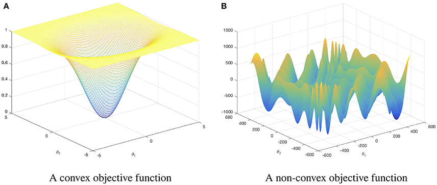
In non-convex functions depending on the starting point, gradient descent will typically be attracted to the first local minima it encounters, so there is no guarantee it will a “good” local minima. In non-convex function shown above, there are a lot of local optima. And the optimization algorithms get stuck in a local optimum rather than find its way to a global optimum. How can we avoid this problem? In logistic regression, the initial cost function is a non-convex function. It is converted to convex function and this guarantees to find the global optimum.
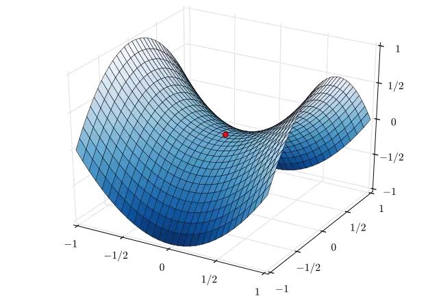
In a neural network, this intuition isn't actually correct. It turns out if we create a neural network, most points of zero gradients are not local optima. Instead, most points of zero gradients in a cost function are saddle points.
In mathematics, a saddle point or minimax point is a point on the surface of the graph of a function where the slopes (derivatives) of orthogonal function components defining the surface become zero (a stationary point) but are not a local extremum on both axes.
So, that's a point where the zero gradients, again. But informally, a function of very high dimensional space, if the gradient is zero, then in each direction it can either be a convex light function or a concave light function. And if we are in, say, a 10,000-dimensional space, then for it to be local optima, all 10,000 directions need to look like the convex function shown above. And so the chance of that happening is maybe very small.
Instead, you're much more likely to get some directions where the curve bends up like so, as well as some directions where the curve function is bending down rather than have them all bend upwards. So that's why in very high-dimensional spaces you're actually much more likely to run into a saddle point like that shown on the right, then the local optimum. That's why this point here, where the derivative is zero, that point is called a saddle point.
If local optima aren't a problem, then what is a problem? It turns out that plateaus can really slow down learning.
a plateau is a region where the derivative is close to zero for a long time.
So if we are at a plateau, then gradient descents will move down the surface, and because the gradient is zero or near zero, the surface is quite flat. And maybe algorithm can actually take a very long time, to slowly find its way off the plateau due to a random perturbation of left or right.
The final takeaways about local optima are
- It is unlikely to get stuck in bad local optima so long if we're training a reasonably large neural network.
- The plateaus can actually make learning pretty slow. And this problem can be solved using algorithms like momentum or RmsProp or Adam.
Gradient Descent in Neural Networks
In the Linear equation that explained above has two paramters (theta 1 and theta 2). Gradient Descent will minimize the cost function (Mean Square error) by updating theta 1 and theta 2.
In Neural Networks there are many weight parameters in different layers to update simultaneously. In order to minimize the loss function, Gradient Descent uses backpropogation to update each weight parameter in each layer of Neural Network.
I hope you liked this tutorial. Do check the following resources:
- So what is the derivative, after all?
- Machine learning course on Coursera by Andrew Ng
- Can gradient descent be applied to non-convex functions?
- Saddle Points
- local minima vs saddle points in deep learning
- Introduction to Gradient Descent Algorithm (along with variants) in Machine Learning
If you have any question or feedback, please do reach out to me by commenting below.
